Introduction to Supervised Learning

Day 1: Introduction

Think of examples

How is data used to make decisions that affect you or your neighbors?

Use whatever resources you like.

Predictive Analytics

A powerful tool to turn data into action.
It works because God made the universe predictable (and successful prediction rewarding), and promised order:
- covenant with Noah that the seasons would continue (Gen 8:22)
- guarantee in Psalms that the sun would rise (Ps 104:19)
- promise to Jeremiah that the sun, moon, and stars would continue (Jer 31:35-36)
Need for wisdom: It can be used for great good and great harm

Power of Predictive Modeling

Medicine: wearable monitor for seizures or falls, detect malaria from blood smears, find effective drug regimens from medical records
Drug Discovery: predict the efficacy of a synthesis plan for a drug
Precision Agriculture: predict effect of micro-climate on plant growth
Urban Planning: forecast resource needs, extreme weather risks, …
Government: classify feedback from constituents
Retail: predict items in a grocery order
Recommendation systems: Amazon, Netflix, YouTube, …
User interfaces: gesture typing, autocomplete / autocorrect

and so much more…

The universe is surprisingly predictable

God created the world with actionable structure
- We gradually learn how to perceive that structure and act within it.
- The better our perceptions align with how the universe is structured, the better our actions
- We can discover that structure by learning to be less surprised by what we see ( = predicting our perceptions)
Perceptions are thus both accurate and fallable.

Predictive modeling technology: Need for wisdom

Potential for great good, but also great harm:
- Lack of fairness in facial recognition, criminal risk, lending, job applicant scoring, …
- Lack of transparency in how “Big Data” systems make conclusions
- Lack of privacy as data is increasingly collected and aggregated
- Amplification of extreme positions in social media, YouTube, etc.
- Oversimplification of human experience
- Hidden human labor
- Illusion of objectivity
- …!

See, for example, Weapons of Math Destruction

Reminders from Statistics

We might wish we had all possible data…
We must acknowledge our uncertainty.
- Our measurements are partial.
- Our inferences sometimes fail (and we may not know it!)
But God made a world with structure that we can learn about even with imperfect tools.

Activity

Teachable Machine

Pick a partner (or two). Decide who’s trainer and who’s tester.

Trainer (needs a laptop):

Go to https://teachablemachine.withgoogle.com/train/image
Train a simple classifier using your webcam. Ideas:
- which hand are you holding up? happy or sad face? looking left or right? two colors?
Don’t worry about making it super accurate.

Tester:

Try out your partner’s classifier (without touching the computer or the same objects).
- Try to find some situations where it works
- Try to write a succinct description of what situations cause it to behave unexpectedly.

We’ll share descriptions.

Supervised Learning and the scikit-learn API

Scikit-Learn (sklearn)

A Python library for machine learning
Provides a consistent API for many different kinds of models
Provides many tools for data preparation, model evaluation, etc.

Model API: `fit`, `predict`

flowchart LR
    A1[("Training Data (X and y)")] --> B{{fit}}
    A2[Model Object] --> B
    B --> FM[Fitted Model]
    FM --> C{{Predict}}
    B2[(New data X)] --> C
    C --> D[("predicted y's")]

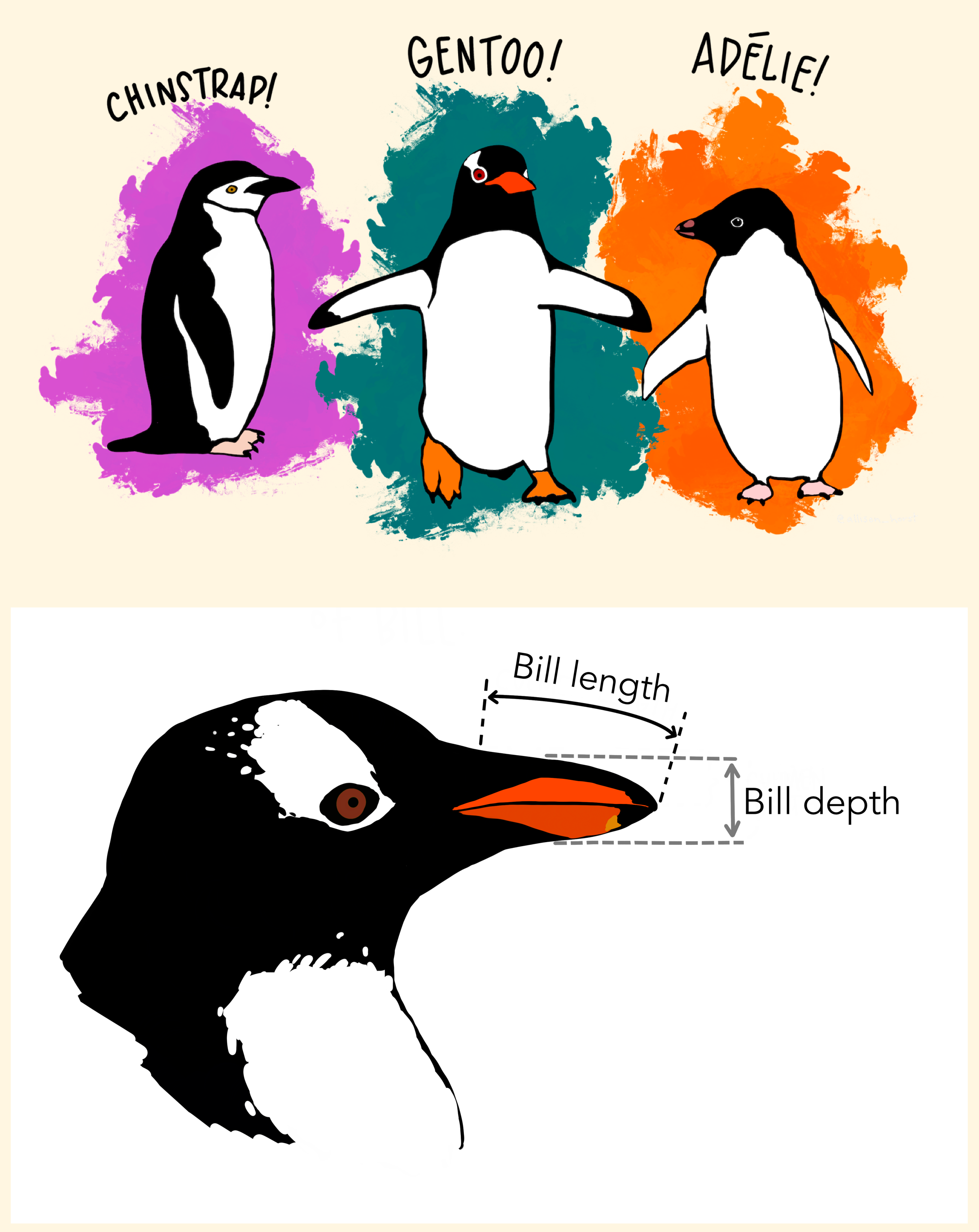
Example: penguins

import pandas as pd
penguins = pd.read_csv("https://raw.githubusercontent.com/allisonhorst/palmerpenguins/main/inst/extdata/penguins.csv")
penguins.info()

<class 'pandas.core.frame.DataFrame'>
RangeIndex: 344 entries, 0 to 343
Data columns (total 8 columns):
 #   Column             Non-Null Count  Dtype  
---  ------             --------------  -----  
 0   species            344 non-null    object 
 1   island             344 non-null    object 
 2   bill_length_mm     342 non-null    float64
 3   bill_depth_mm      342 non-null    float64
 4   flipper_length_mm  342 non-null    float64
 5   body_mass_g        342 non-null    float64
 6   sex                333 non-null    object 
 7   year               344 non-null    int64  
dtypes: float64(4), int64(1), object(3)
memory usage: 21.6+ KB

penguins_simple = penguins[['bill_depth_mm', 'bill_length_mm', 'species']].dropna().copy()

Which species is each penguin?

from sklearn.neighbors import KNeighborsClassifier
model = KNeighborsClassifier(n_neighbors=1).fit(
    X=penguins_simple[['bill_depth_mm', 'bill_length_mm']],
    y=penguins_simple['species'])

penguins_simple['predicted_species'] = model.predict(
    X=penguins_simple[['bill_depth_mm', 'bill_length_mm']])
penguins_simple.head()

	bill_depth_mm	bill_length_mm	species	predicted_species
0	18.7	39.1	Adelie	Adelie
1	17.4	39.5	Adelie	Adelie
2	18.0	40.3	Adelie	Adelie
4	19.3	36.7	Adelie	Adelie
5	20.6	39.3	Adelie	Adelie

Are those predictions are good?

penguins_simple.groupby(['species', 'predicted_species'], as_index=False).size()

	species	predicted_species	size
0	Adelie	Adelie	151
1	Chinstrap	Chinstrap	68
2	Gentoo	Gentoo	123

from sklearn.metrics import accuracy_score
accuracy_score(
    y_true=penguins_simple['species'],
    y_pred=penguins_simple['predicted_species'])

1.0

Well, of course…

Why should we be unsurprised that this works?

Train-test split!

flowchart LR
    A1[("All training data")] --> B{{Split}}
    B --> A2[("Training data")]
    B --> A3[("Test data")]
    A2 --> C{{Fit}}
    A3 -->|NEVER!| C
    C --> D[("Fitted model")]

import numpy as np
np.random.seed(0)
penguins_simple["use_for_training"] = np.random.rand(len(penguins_simple)) < 0.5
penguins_train = penguins_simple.query("use_for_training").copy()
penguins_test = penguins_simple.query("not use_for_training").copy()    
print(f"{len(penguins_train)} training penguins, {len(penguins_test)} test penguins")

171 training penguins, 171 test penguins

Note: Later we’ll learn about the train_test_split function, which does this for us.

Train on the training set

model = KNeighborsClassifier(n_neighbors=1).fit(
    X=penguins_train[['bill_depth_mm', 'bill_length_mm']],
    y=penguins_train['species'])

How does it do?

penguins_train['predicted_species'] = model.predict(
    X=penguins_train[['bill_depth_mm', 'bill_length_mm']])
penguins_train.groupby(['species', 'predicted_species'], as_index=False).size()

	species	predicted_species	size
0	Adelie	Adelie	69
1	Chinstrap	Chinstrap	39
2	Gentoo	Gentoo	63

penguins_test['predicted_species'] = model.predict(
    X=penguins_test[['bill_depth_mm', 'bill_length_mm']])
penguins_test.groupby(['species', 'predicted_species'], as_index=False).size()

	species	predicted_species	size
0	Adelie	Adelie	81
1	Adelie	Chinstrap	1
2	Chinstrap	Adelie	2
3	Chinstrap	Chinstrap	26
4	Chinstrap	Gentoo	1
5	Gentoo	Chinstrap	6
6	Gentoo	Gentoo	54

accuracy_score(
    y_true=penguins_test['species'],
    y_pred=penguins_test['predicted_species'])

0.9415204678362573

Other kinds of models

Nearest Neighbors (KNeighborsClassifier)
Decision Trees (DecisionTreeClassifier) and Random Forests (RandomForestClassifier)
Linear Models (LogisticRegression, yes it’s a classifier)
Neural Networks (MLPClassifier)
Boosting methods (HistGradientBoostingClassifier)

Many models, same API

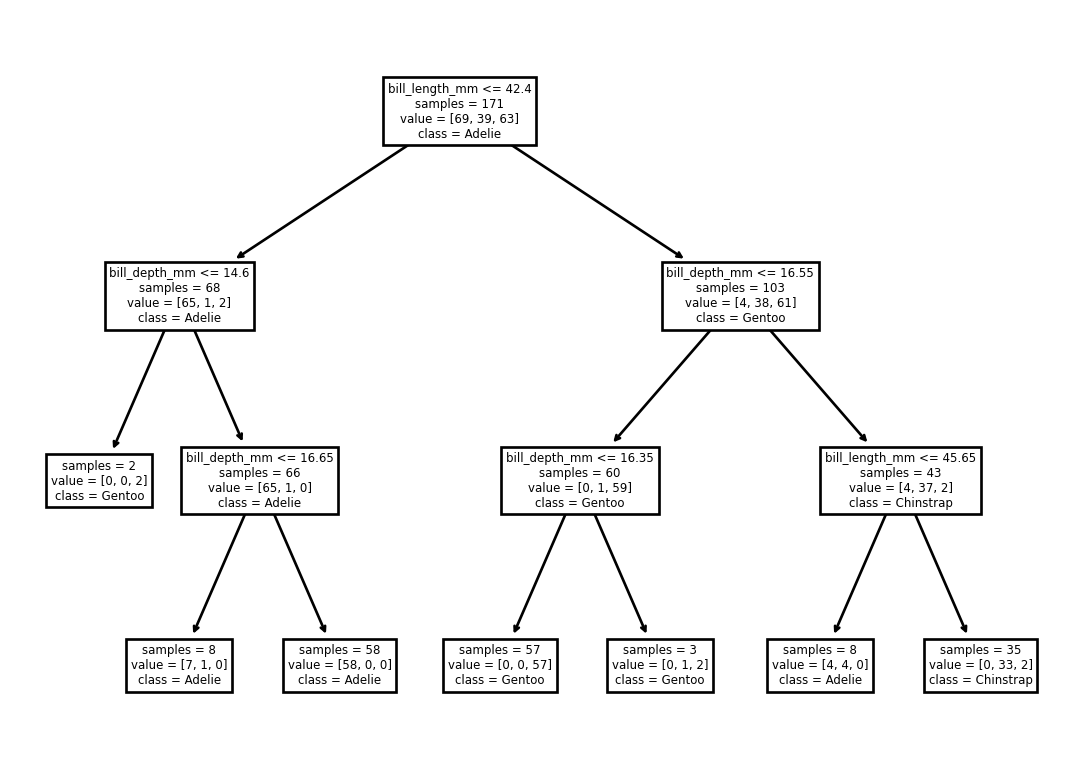
Decision tree:

from sklearn.tree import DecisionTreeClassifier, plot_tree
model = DecisionTreeClassifier(max_depth=3).fit(
        X=penguins_train[['bill_depth_mm', 'bill_length_mm']],
        y=penguins_train['species'])
model.score(
    X=penguins_test[['bill_depth_mm', 'bill_length_mm']],
    y=penguins_test['species'])

0.9122807017543859

What does that tree do?

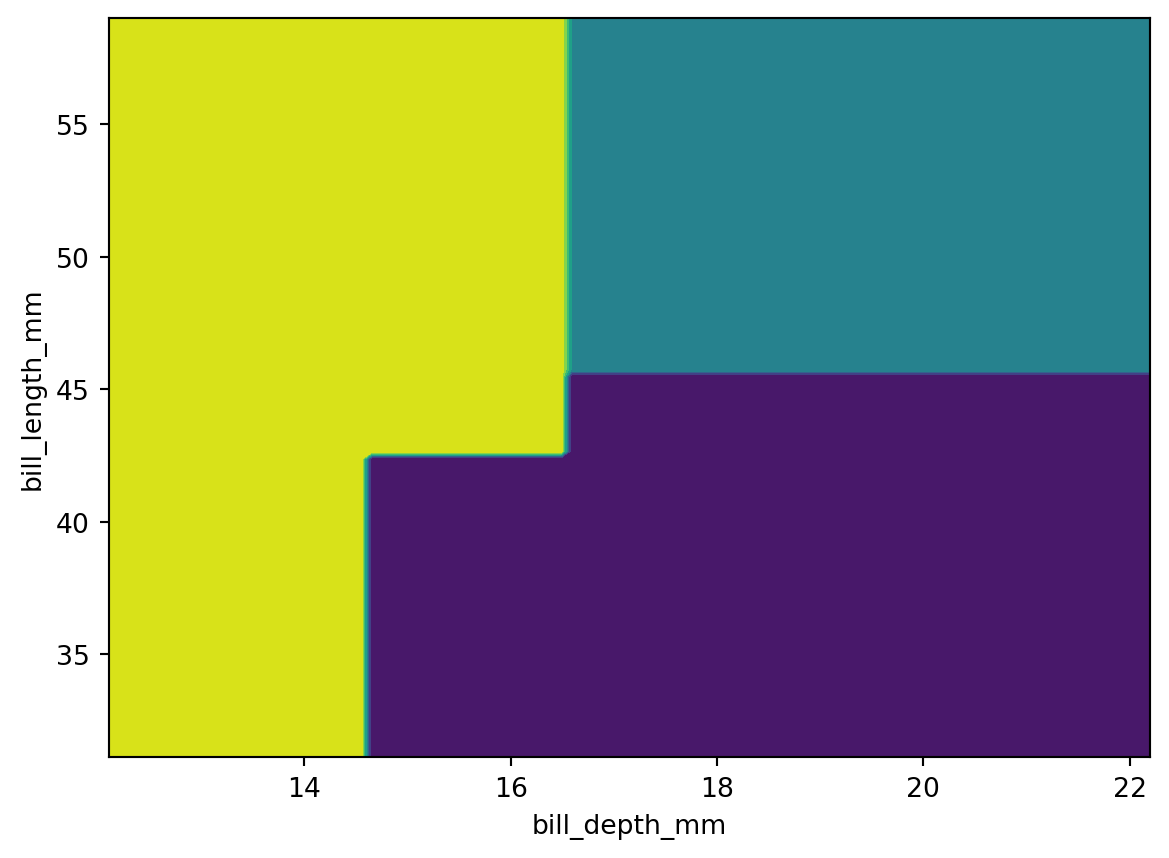
Linear Model (Logistic Regression)

from sklearn.linear_model import LogisticRegression
model = LogisticRegression().fit(
    X=penguins_train[['bill_depth_mm', 'bill_length_mm']],
    y=penguins_train['species'])

model.coef_

array([[ 1.91703649, -0.89183601],
       [ 0.39297577,  0.28951405],
       [-2.31001227,  0.60232196]])

model.score(
    X=penguins_test[['bill_depth_mm', 'bill_length_mm']],
    y=penguins_test['species'])

0.9707602339181286

Neural Network

from sklearn.neural_network import MLPClassifier
model = MLPClassifier(hidden_layer_sizes=(10, 10)).fit(
    X=penguins_train[['bill_depth_mm', 'bill_length_mm']],
    y=penguins_train['species'])

/usr/local/Caskroom/miniconda/base/envs/fa22/lib/python3.10/site-packages/sklearn/neural_network/_multilayer_perceptron.py:702: ConvergenceWarning:

Stochastic Optimizer: Maximum iterations (200) reached and the optimization hasn't converged yet.

model.score(
    X=penguins_test[['bill_depth_mm', 'bill_length_mm']],
    y=penguins_test['species'])

0.38596491228070173

Wednesday Slides

Recall

What does fit do?
What does predict do?
Why did we get an accuracy_score of 1.0? What did we do wrong?
What should you never do with the test set?

Types of Learning from Data

Supervised Learning: Filling in a label for each item based on features
- Classification: Labels are discrete (e.g. penguin species, spam/not spam, which word was swiped, …)
- Regression: Labels are continuous (e.g. sale price, seconds of video watched, …)
  - Forecasting: predict how a sequence will continue (future observations)
Unsupervised Learning: Finding relationships between items, doesn’t need labels
- Clustering: Grouping similar items (e.g. customer segments, …)
- Dimensionality Reduction: Finding a lower-dimensional representation of data (e.g. word embeddings, …)

We’ll focus on supervised learning and clustering in this course. Others:

Reinforcement Learning: Learning to take actions to maximize a reward (e.g. game playing, robotics, …)
Self-supervised learning: turning an unsupervised problem into a supervised one (e.g. predicting the next word in a sentence)
Statistical inference: fill in summary statistics (we wanted a population but only got a sample)
Causal inference: fill in counterfactuals (what if?)

Regression Example 1

Concrete Mixture Strength

From Applied Predictive Modeling (M. Kuhn and Johnson 2013), chapter 10.

from sklearn.datasets import fetch_openml
concrete = fetch_openml(data_id=4353)
concrete_all = concrete['data'].copy()

Original column names:
['Cement (component 1)(kg in a m^3 mixture)', 'Blast Furnace Slag (component 2)(kg in a m^3 mixture)', 'Fly Ash (component 3)(kg in a m^3 mixture)', 'Water  (component 4)(kg in a m^3 mixture)', 'Superplasticizer (component 5)(kg in a m^3 mixture)', 'Coarse Aggregate  (component 6)(kg in a m^3 mixture)', 'Fine Aggregate (component 7)(kg in a m^3 mixture)', 'Age (day)', 'Concrete compressive strength(MPa. megapascals)']

# clean up column names: remove everything after the first parenthesis, replace spaces with underscores
concrete_all.columns = [
    col.split('(', 1)[0].strip().replace(' ', '_').lower()
    for col in concrete_all.columns]
concrete_all = concrete_all.rename(columns={
    'concrete_compressive_strength': 'strength',
    'blast_furnace_slag': 'slag',
})
concrete_all.info()

<class 'pandas.core.frame.DataFrame'>
RangeIndex: 1030 entries, 0 to 1029
Data columns (total 9 columns):
 #   Column            Non-Null Count  Dtype  
---  ------            --------------  -----  
 0   cement            1030 non-null   float64
 1   slag              1030 non-null   float64
 2   fly_ash           1030 non-null   float64
 3   water             1030 non-null   float64
 4   superplasticizer  1030 non-null   float64
 5   coarse_aggregate  1030 non-null   float64
 6   fine_aggregate    1030 non-null   float64
 7   age               1030 non-null   float64
 8   strength          1030 non-null   float64
dtypes: float64(9)
memory usage: 72.5 KB

Concrete Mixture Strength data

concrete_all.head()

	cement	slag	water	superplasticizer	coarse_aggregate	fine_aggregate	age	strength
0	540.0	0.0	162.0	2.5	1040.0	676.0	28.0	79.99
1	540.0	0.0	162.0	2.5	1055.0	676.0	28.0	61.89
2	332.5	142.5	228.0	0.0	932.0	594.0	270.0	40.27
3	332.5	142.5	228.0	0.0	932.0	594.0	365.0	41.05
4	198.6	132.4	192.0	0.0	978.4	825.5	360.0	44.30

Modeling Workflow

Step 1: Define the problem

What are you trying to predict?
- terms: target, response, label
What data do you have?
- terms: features, predictors, covariates
What metrics will indicate success? (Measure success in multiple ways!)
- terms: loss, error, score, metric
- penguins example: accuracy (perhaps broken down by species)

Concrete example:

Task: predict concrete strength (MPa) from mixture ingredients
Target: concrete strength
Features: mixture ingredients (cement, slag, ash, water, …)
Metric: how close are the predictions to the actual strength?

Step 2: Explore the data

What is the structure of the data?
What are the distributions of the features and target?
Anything unexpected? (e.g. missing values, outliers, …): make lots of plots!

Concrete example:

import plotly.express as px
px.histogram(concrete_all, x='strength', nbins=30)

px.histogram(concrete_all, x='age', nbins=30)

# Do we have duplicates of any mixtures that differ only in age and strength?
other_columns = [col for col in concrete_all.columns if col not in ['age', 'strength']]
concrete_all.groupby(other_columns, as_index=False).size().sort_values(by='size', ascending=False).head(10)

	cement	slag	fly_ash	water	superplasticizer	coarse_aggregate	fine_aggregate	size
356	362.6	189.0	0.0	164.9	11.6	944.7	755.8	20
393	425.0	106.3	0.0	153.5	16.5	852.1	887.1	15
398	446.0	24.0	79.0	162.0	11.6	967.0	712.0	12
413	500.0	0.0	0.0	200.0	0.0	1125.0	613.0	8
355	359.0	19.0	141.0	154.0	10.9	942.0	801.0	8
426	540.0	0.0	0.0	173.0	0.0	1125.0	613.0	7
421	525.0	0.0	0.0	189.0	0.0	1125.0	613.0	7
342	339.0	0.0	0.0	197.0	0.0	968.0	781.0	7
367	380.0	95.0	0.0	228.0	0.0	932.0	594.0	6
147	198.6	132.4	0.0	192.0	0.0	978.4	825.5	6

We’ll need to address this later.

Are they all the same total weight?

concrete_all[other_columns].sum(axis=1).describe()

count    1030.000000
mean     2343.523398
std        65.365356
min      2194.600000
25%      2291.150000
50%      2349.100000
75%      2390.400000
max      2551.000000
dtype: float64

Step 3: Split the data

So we can evaluate the model.

Splitting concrete data

from sklearn.model_selection import train_test_split

concrete_train, concrete_test = train_test_split(concrete_all, random_state=0, test_size=0.2)
print(f"{len(concrete_train)} training mixtures, {len(concrete_test)} test mixtures")

824 training mixtures, 206 test mixtures

Careful: we just duplicated some mixtures in both sets (measurements at different ages).

Step 4: Feature Engineering

Sometimes the features are already in a useful form, but sometimes we can get more useful features by transforming or combining the existing features.

Examples:

ratios of ingredients (e.g., coarse aggregate / fine aggregate)
log of age (influence of a day decreases as age increases)
polynomial features (e.g. \(x^2\))
product of two features (interactions)
date features (e.g., day of week, month)
replace rare categories with “other”

We’ll skip this for concrete for now.

Step 5: Train (fit) and evaluate some models

Pick a model (or several) that’s appropriate for the task and data
Fit the model to the training data
Evaluate the model on the test data

Some models may require special preparation of the data:

Missing values
Categorical variables
Scaling
Feature engineering

Step 5: a linear model for concrete

from sklearn.linear_model import LinearRegression
feature_columns = [col for col in concrete_train.columns if col != 'strength']
model = LinearRegression().fit(
    X=concrete_train[feature_columns],
    y=concrete_train['strength'])

concrete_test['predicted_strength'] = model.predict(
    X=concrete_test[feature_columns])

Metrics: Were those predictions good?

from sklearn.metrics import mean_absolute_error, mean_absolute_percentage_error, mean_squared_error, r2_score

def evaluate(y_true, y_pred):
    return pd.Series({
        'MAE': mean_absolute_error(y_true, y_pred),
        'MAPE': mean_absolute_percentage_error(y_true, y_pred),
        'R^2': r2_score(y_true, y_pred),
    })

def evaluate_df(df):
    return evaluate(df['strength'], df['predicted_strength'])

evaluate_df(concrete_test).to_frame('test')

	test
MAE	7.864642
MAPE	0.331604
R^2	0.636961

MAE: Mean Absolute Error (“predictions are usually off by xxx MPa”)
MAPE: Mean Absolute Percent Error (“predictions are usually off by yy%”)
Traditional R^2 (fraction of variance explained)

Note: Above, we defined a function to evaluate these errors on any model. That way we can evaluate many models in the same way.

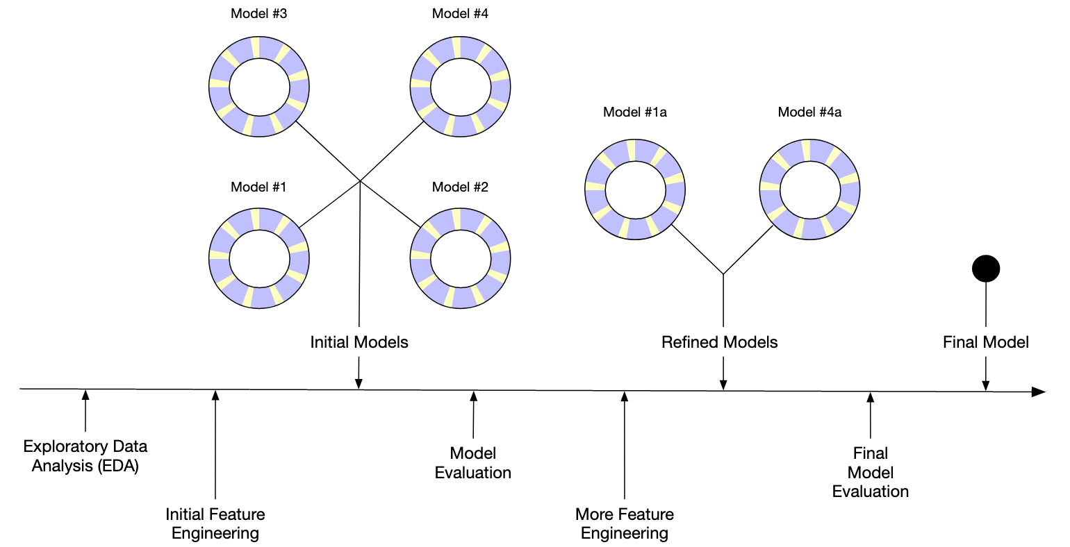
Step 6: Tune the model

Try different models and hyperparameters
Try different feature engineering
Analyze model errors (more EDA)
Repeat steps 4-6 until model is good enough

EDA on model errors for Concrete

concrete_test['error'] = concrete_test['strength'] - concrete_test['predicted_strength']
px.histogram(concrete_test, x='error', nbins=30)

Does the model do better or worse for certain ranges?

px.scatter(
    concrete_test,
    x='strength', y='error',
    trendline='ols',
    labels={
        'strength': 'Strength (MPa)',
        'error': 'Error (MPa)',
    },
)

concrete_test['strength_bin'] = pd.cut(concrete_test['strength'], bins=5)
concrete_test.groupby('strength_bin', as_index=False).apply(evaluate_df)

	strength_bin	MAE	MAPE	R^2
0	(4.495, 19.516]	9.000968	0.848740	-5.671546
1	(19.516, 34.462]	5.808164	0.213878	-2.287072
2	(34.462, 49.408]	8.305960	0.201023	-5.271035
3	(49.408, 64.354]	8.740660	0.154203	-4.768868
4	(64.354, 79.3]	11.762144	0.164826	-7.339047

concrete_test['age_bin'] = pd.cut(concrete_test['age'], bins=3)
concrete_test.groupby('age_bin', as_index=False).apply(evaluate_df)

	age_bin	MAE	MAPE	R^2
0	(2.638, 123.667]	7.760751	0.339492	0.652625
1	(123.667, 244.333]	6.864034	0.188294	0.568809
2	(244.333, 365.0]	11.220562	0.268660	-2.173470

Any relationships with other features?

px.scatter(
    concrete_test,
    x='water', y='error', trendline='ols',
)

We’re not seeing any clear overall patterns. Which mixtures are we worst at predicting? (ask a domain expert about these)

concrete_test.sort_values(by='error').head(5)

	cement	slag	fly_ash	water	superplasticizer	coarse_aggregate	fine_aggregate	age	strength	predicted_strength	error	strength_bin	age_bin
477	446.0	24.0	79.0	162.0	11.6	967.0	712.0	3.0	23.35	50.426023	-27.076023	(19.516, 34.462]	(2.638, 123.667]
85	379.5	151.2	0.0	153.9	15.9	1134.3	605.0	3.0	28.60	52.987434	-24.387434	(19.516, 34.462]	(2.638, 123.667]
622	307.0	0.0	0.0	193.0	0.0	968.0	812.0	365.0	36.15	59.850056	-23.700056	(34.462, 49.408]	(244.333, 365.0]
604	339.0	0.0	0.0	197.0	0.0	968.0	781.0	365.0	38.89	62.387515	-23.497515	(34.462, 49.408]	(244.333, 365.0]
294	168.9	42.2	124.3	158.3	10.8	1080.8	796.2	3.0	7.40	28.205935	-20.805935	(4.495, 19.516]	(2.638, 123.667]

concrete_test.sort_values(by='error').tail(5)

	cement	slag	fly_ash	water	superplasticizer	coarse_aggregate	fine_aggregate	age	strength	predicted_strength	error	strength_bin	age_bin
358	277.2	97.8	24.5	160.7	11.2	1061.7	782.5	100.0	66.95	48.291387	18.658613	(64.354, 79.3]	(2.638, 123.667]
828	522.0	0.0	0.0	146.0	0.0	896.0	896.0	28.0	74.99	53.777042	21.212958	(64.354, 79.3]	(2.638, 123.667]
356	277.2	97.8	24.5	160.7	11.2	1061.7	782.5	28.0	63.14	39.996732	23.143268	(49.408, 64.354]	(2.638, 123.667]
8	266.0	114.0	0.0	228.0	0.0	932.0	670.0	28.0	45.85	19.463945	26.386055	(34.462, 49.408]	(2.638, 123.667]
14	304.0	76.0	0.0	228.0	0.0	932.0	670.0	28.0	47.81	19.859987	27.950013	(34.462, 49.408]	(2.638, 123.667]

Concrete: try a different model

e.g., random forest

from sklearn.ensemble import RandomForestRegressor
model = RandomForestRegressor(n_estimators=100, random_state=0)

Your turn: how well does a Random Forest model do on the test set?

Step 7: Deploy the model

Often called “inference” (as opposed to “training”)

Use the model to make predictions on new data as it arrives
Monitor the model’s performance over time
Retrain the model periodically