Imports …
import pandas as pdimport numpy as npfrom sklearn.metrics import accuracy_scoreimport plotly.express as pximport matplotlib.pyplot as pltimport plotly.io as pio= "plotly_white"
Example: Blood test for autism?
We’ll use an example from a 2017 PLOS Computational Biology paper . Download the data .
Typically autism is diagnosed by behavioral symptoms
If we could diagnose autism from a blood test, we could diagnose it earlier
The data has units on the second row, so we’ll skip that row.
= pd.read_csv("data/autism.csv" , skiprows= [1 ])
Exploratory Data Analysis (EDA)
What do these metabolites look like?
= (= "Group" , var_name= "Measure" , value_name= "value" )"Group != 'SIB' and Measure != 'Vineland ABC'" )= "value" ,= "Measure" ,= "Group"
Exploratory Data Analysis (EDA)
EDA
This plot helps us compare different metabolites within each group.
Better question for predictive task: Which of these metabolites help us distinguish autism?
Approach:
easier to compare within a plot than across a facet, so switch y variable to Group.
absolute values don’t matter much, so let each metabolite have its own x scale.
plotly boxplots don’t show up well when small, so switch to a ridgeline plot
= "value" ,= "Group" ,= "Measure" , facet_col_wrap= 5 = "positive" , width= 3 , points= False )= None )lambda a: a.update(text= a.text.split("=" , 1 )[- 1 ], font_size= 10 ))
Train-test split
from sklearn.model_selection import train_test_split= train_test_split(data, test_size= 0.25 , random_state= 123 )print ("Training set shape: {} " .format (train.shape))print ("Test set shape: {} " .format (test.shape))
Training set shape: (119, 25)
Test set shape: (40, 25)
First Model: guessing most common
What if we always guessed the most common outcome?
from sklearn.dummy import DummyClassifier= DummyClassifier(strategy= "most_frequent" ).fit(= train[feature_columns],= train[target_column]"pred_most_common" ] = most_common.predict(test[feature_columns])"pred_most_common" ])
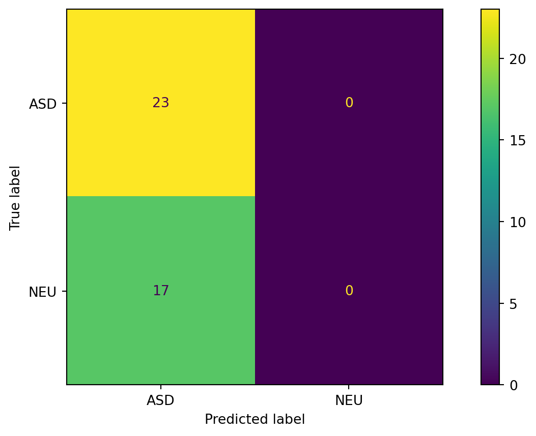
Confusion Matrix for most common
from sklearn.metrics import confusion_matrix, ConfusionMatrixDisplay= most_common,= test[feature_columns],= test[target_column],= [positive_outcome, negative_outcome]
Computing these automatically
Now we can compute them (see docs on classification metrics )
from sklearn.metrics import classification_reportprint (classification_report(= test[target_column],= test["pred_uniform" ],
              precision    recall  f1-score   support

         ASD       0.65      0.48      0.55        23
         NEU       0.48      0.65      0.55        17

    accuracy                           0.55        40
   macro avg       0.56      0.56      0.55        40
weighted avg       0.58      0.55      0.55        40
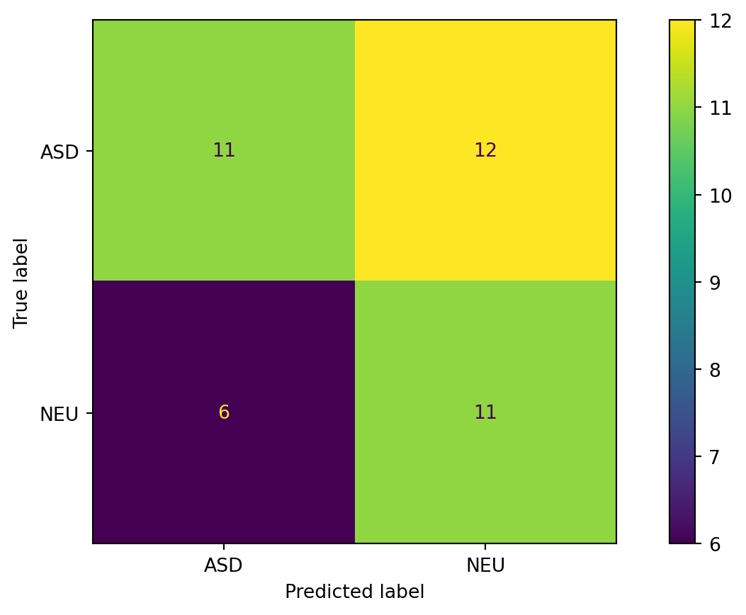
Let’s compute these quantities straight from the confusion matrix.
from sklearn.metrics import confusion_matrix= confusion_matrix(= test[target_column],= test["pred_uniform" ],= [negative_outcome, positive_outcome]= tp + fn= tn + fpprint (f"Accuracy: { (tp + tn) / (num_positives + num_negatives):.2f} " )print (f"False positive rate: { fp / num_negatives:.2f} " )print (f"False negative rate: { fn / num_positives:.2f} " )print (f"Sensitivity / recall: { tp / num_positives:.2f} " )print (f"Specificity: { tn / (tn + fp):.2f} " )print (f"Precision: { tp / (tp + fp):.2f} " )
Accuracy: 0.55
False positive rate: 0.35
False negative rate: 0.52
Sensitivity / recall: 0.48
Specificity: 0.65
Precision: 0.65
Decision Tree
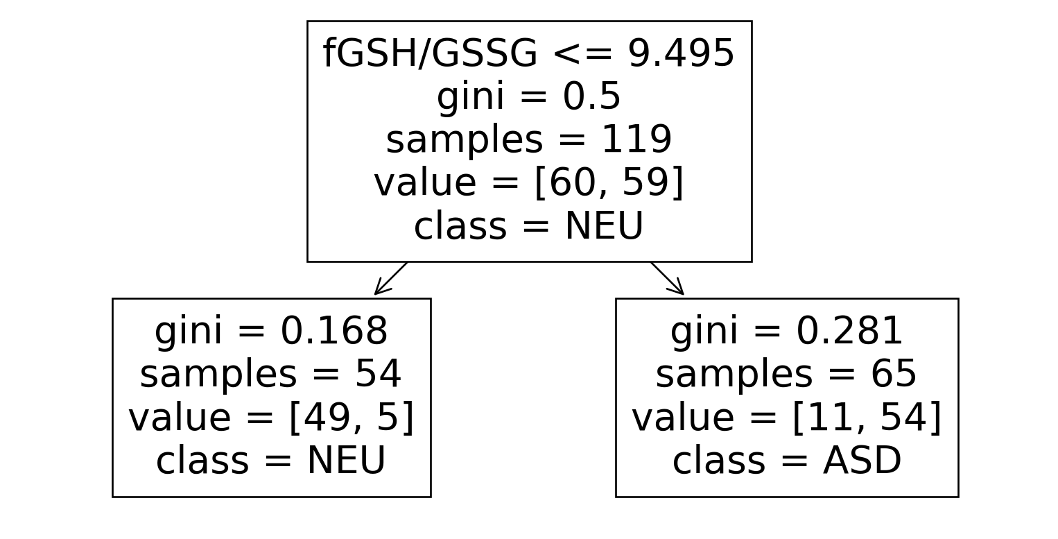
from sklearn.tree import DecisionTreeClassifier= DecisionTreeClassifier(max_depth= 1 ).fit(= train[feature_columns],= train[target_column]"pred_tree" ] = tree.predict(train[feature_columns])print ("Training accuracy: " , accuracy_score(train[target_column], train["pred_tree" ]))
Training accuracy: 0.865546218487395
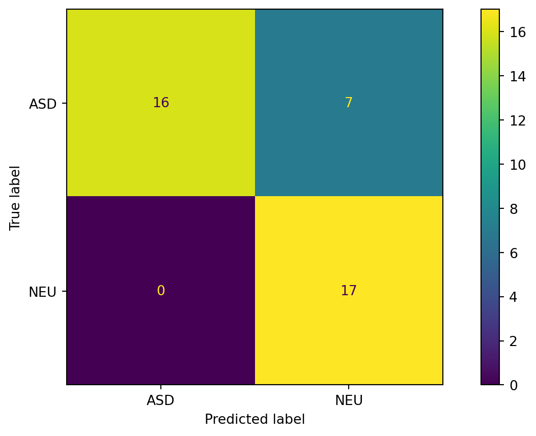
"pred_tree" ] = tree.predict(test[feature_columns])print ("Test accuracy: " , accuracy_score(test[target_column], test["pred_tree" ]))
Confusion Matrix
= tree,= test[feature_columns],= test[target_column],= [positive_outcome, negative_outcome]
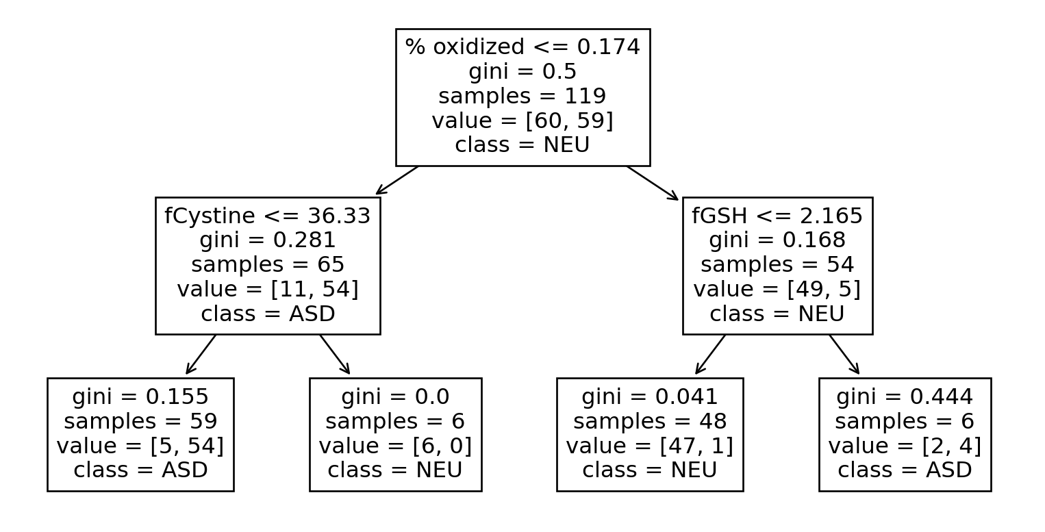
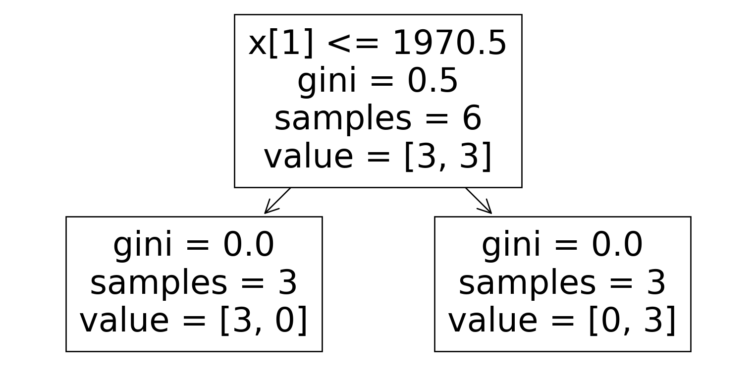
What does the tree look like?
from sklearn.tree import plot_tree= feature_columns, class_names= [negative_outcome, positive_outcome]);
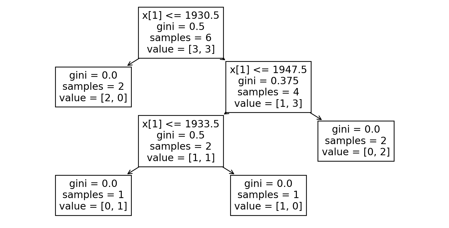
Go Deeper
= DecisionTreeClassifier(max_depth= 2 ).fit(= train[feature_columns],= train[target_column]"pred_tree" ] = tree.predict(train[feature_columns])print ("Training accuracy: " , accuracy_score(train[target_column], train["pred_tree" ]))
Training accuracy: 0.9327731092436975
= feature_columns, class_names= [negative_outcome, positive_outcome]);
"pred_tree" ] = tree.predict(test[feature_columns])print ("Test accuracy: " , accuracy_score(test[target_column], test["pred_tree" ]))
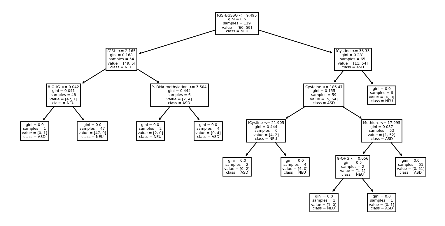
Even Deeper
= DecisionTreeClassifier(max_depth= 30 ).fit(= train[feature_columns],= train[target_column]"pred_tree" ] = tree.predict(train[feature_columns])print ("Training accuracy: " , accuracy_score(train[target_column], train["pred_tree" ]))
= feature_columns, class_names= [negative_outcome, positive_outcome]);
What do you think the test accuracy will be?
"pred_tree" ] = tree.predict(test[feature_columns])print ("Test accuracy: " , accuracy_score(test[target_column], test["pred_tree" ]))
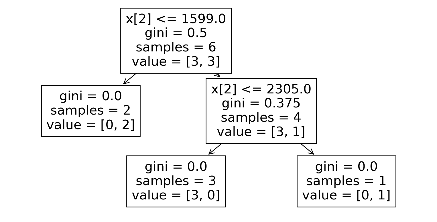
What decisions can be made at each node
Continuous variables: compare one feature against a threshold value; if comparison is true go right, else go left
Categorical variables: if is one of a set of categories, go right, else left
At leaf nodes:
regression tree: compute the mean value of items there, predict that.
classification tree: compute the proportion of each category for items there
predict the most common category
or: predict that unseen items will follow the same proportions
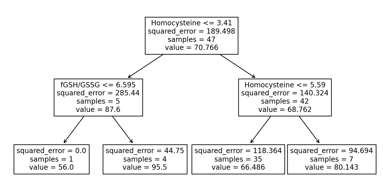
Example of a Regression Tree
We’ll try predicting the “Vineland ABC” score from the metabolites (for just the ASD children).
We’ll skip the usual train-test split because we’re just showing what the tree looks like.
from sklearn.tree import DecisionTreeRegressor= autism.query("Group == 'ASD'" ).dropna().copy()= DecisionTreeRegressor(max_depth= 2 ).fit(= just_asd[feature_columns],= just_asd["Vineland ABC" ]
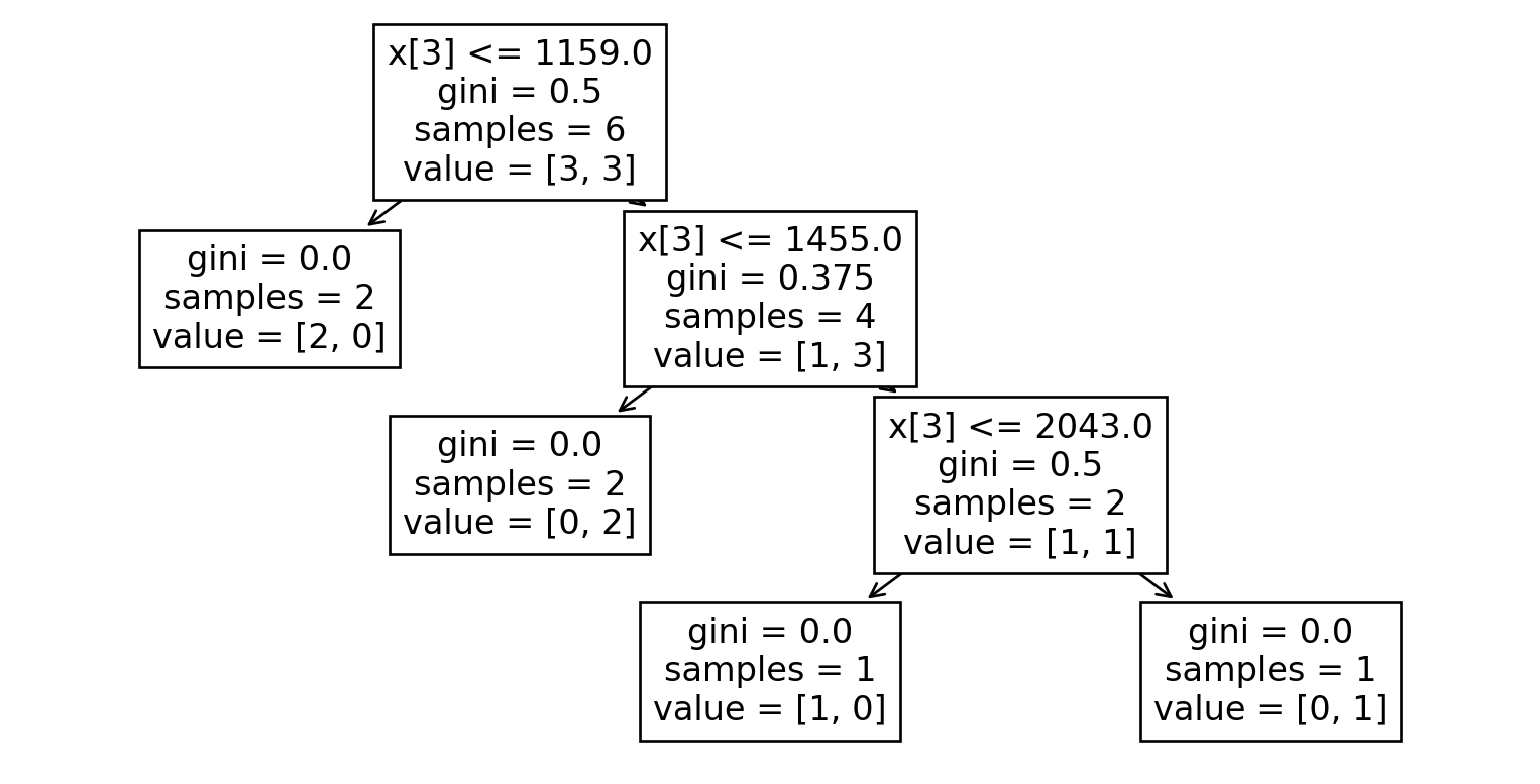
What a regression tree looks like
= feature_columns);
Training Data (Classification Tree)
1734
Attchd
No
1422
Attchd
Yes
1464
Attchd
Yes
2320
Detchd
Yes
2290
Detchd
No
1969
Detchd
No
1973
Twnhs
No
1980
Duplex
No
2002
OneFam
Yes
1962
OneFam
No
1994
OneFam
Yes
1994
OneFam
Yes
1367
TwnhsE
Yes
1512
OneFam
Yes
1149
OneFam
No
796
OneFam
No
1264
OneFam
Yes
1314
OneFam
No
932
OneFam
No
1242
OneFam
Yes
1668
OneFam
No
1092
TwoFmCon
No
1226
TwnhsE
Yes
2418
OneFam
Yes
864
OneFam
No
1434
OneFam
No
1196
OneFam
No
1720
OneFam
Yes
2787
Duplex
Yes
1586
Twnhs
Yes
1900
Detchd
No
2006
Attchd
Yes
1929
Detchd
Yes
1940
Detchd
No
1970
Attchd
Yes
1916
Detchd
No
2000
OneFam
Yes
1967
OneFam
No
1974
OneFam
Yes
1997
OneFam
Yes
1956
OneFam
No
1948
OneFam
No
2005
OneFam
Yes
1950
OneFam
Yes
1937
OneFam
No
1915
OneFam
No
1980
OneFam
Yes
1971
OneFam
No
1403
OneFam
Yes
1342
OneFam
No
2161
OneFam
Yes
1092
Twnhs
No
1852
OneFam
Yes
1578
OneFam
No
1959
OneFam
Yes
1914
OneFam
No
1931
OneFam
Yes
2001
OneFam
Yes
1930
OneFam
No
1936
OneFam
No
1502
1923
OneFam
Detchd
1561
1960
OneFam
Attchd
2650
1967
Duplex
Other
1328
1959
OneFam
Attchd
3228
1992
OneFam
Attchd
1774
1900
OneFam
Other
Training Data (Regression Tree)
1734
Attchd
126.0
1422
Attchd
179.6
1464
Attchd
282.9
2320
Detchd
259.5
2290
Detchd
122.5
1969
Detchd
141.0
1973
Twnhs
119.5
1980
Duplex
144.0
2002
OneFam
220.0
1962
OneFam
130.0
1994
OneFam
193.5
1994
OneFam
301.5
1367
TwnhsE
192.0
1512
OneFam
231.0
1149
OneFam
127.0
796
OneFam
85.0
1264
OneFam
167.5
1314
OneFam
145.0
932
OneFam
124.0
1242
OneFam
175.5
1668
OneFam
135.0
1092
TwoFmCon
55.0
1226
TwnhsE
211.5
2418
OneFam
341.0
864
OneFam
133.5
1434
OneFam
157.0
1196
OneFam
128.0
1720
OneFam
188.0
2787
Duplex
269.5
1586
Twnhs
170.0
1900
Detchd
114.0
2006
Attchd
325.0
1929
Detchd
230.0
1940
Detchd
155.0
1970
Attchd
240.1
1916
Detchd
135.0
2000
OneFam
327.0
1967
OneFam
134.5
1974
OneFam
260.0
1997
OneFam
210.0
1956
OneFam
131.0
1948
OneFam
138.0
2005
OneFam
415.0
1950
OneFam
257.0
1937
OneFam
119.5
1915
OneFam
123.0
1980
OneFam
204.0
1971
OneFam
119.5
1403
OneFam
202.0
1342
OneFam
105.0
2161
OneFam
230.5
1092
Twnhs
85.5
1852
OneFam
230.0
1578
OneFam
133.0
1959
OneFam
200.0
1914
OneFam
67.0
1931
OneFam
169.5
2001
OneFam
421.2
1930
OneFam
110.0
1936
OneFam
115.0
1502
1923
OneFam
Detchd
1561
1960
OneFam
Attchd
2650
1967
Duplex
Other
1328
1959
OneFam
Attchd
3228
1992
OneFam
Attchd
1774
1900
OneFam
Other
Evaluation
Here’s the test set with labels:
1502
1923
OneFam
Detchd
Yes
165.000000
1561
1960
OneFam
Attchd
Yes
193.000000
2650
1967
Duplex
Other
Yes
160.000000
1328
1959
OneFam
Attchd
Yes
170.000000
3228
1992
OneFam
Attchd
Yes
430.000000
1774
1900
OneFam
Other
No
87.000000
Compute your accuracy and MAE.
Reference Results
Here’s what classification trees look like for each dataset:
1734
Attchd
No
1422
Attchd
Yes
1464
Attchd
Yes
2320
Detchd
Yes
2290
Detchd
No
1969
Detchd
No
1973
Twnhs
No
1980
Duplex
No
2002
OneFam
Yes
1962
OneFam
No
1994
OneFam
Yes
1994
OneFam
Yes
1367
TwnhsE
Yes
1512
OneFam
Yes
1149
OneFam
No
796
OneFam
No
1264
OneFam
Yes
1314
OneFam
No
932
OneFam
No
1242
OneFam
Yes
1668
OneFam
No
1092
TwoFmCon
No
1226
TwnhsE
Yes
2418
OneFam
Yes
864
OneFam
No
1434
OneFam
No
1196
OneFam
No
1720
OneFam
Yes
2787
Duplex
Yes
1586
Twnhs
Yes
1900
Detchd
No
2006
Attchd
Yes
1929
Detchd
Yes
1940
Detchd
No
1970
Attchd
Yes
1916
Detchd
No
2000
OneFam
Yes
1967
OneFam
No
1974
OneFam
Yes
1997
OneFam
Yes
1956
OneFam
No
1948
OneFam
No
2005
OneFam
Yes
1950
OneFam
Yes
1937
OneFam
No
1915
OneFam
No
1980
OneFam
Yes
1971
OneFam
No
1403
OneFam
Yes
1342
OneFam
No
2161
OneFam
Yes
1092
Twnhs
No
1852
OneFam
Yes
1578
OneFam
No
1959
OneFam
Yes
1914
OneFam
No
1931
OneFam
Yes
2001
OneFam
Yes
1930
OneFam
No
1936
OneFam
No
1502
1923
OneFam
Detchd
0.300000
Yes
Yes
No
Yes
No
No
Yes
No
No
No
No
1561
1960
OneFam
Attchd
0.600000
Yes
Yes
No
Yes
No
Yes
Yes
No
Yes
No
Yes
2650
1967
Duplex
Other
0.700000
Yes
Yes
No
Yes
Yes
Yes
Yes
No
No
Yes
Yes
1328
1959
OneFam
Attchd
0.500000
Yes
Yes
No
No
Yes
No
Yes
No
Yes
No
Yes
3228
1992
OneFam
Attchd
1.000000
Yes
Yes
Yes
Yes
Yes
Yes
Yes
Yes
Yes
Yes
Yes
1774
1900
OneFam
Other
0.300000
No
No
No
Yes
No
Yes
No
No
No
Yes
No