Bayesian Networks: a short introduction
Probabilistic Graphical Models
Maybe we can use a graphical representation that helps us simplify that probability?
Several options: Markov Hidden Models, Bayesian networks…
Bayesian networks take advantage on the conditional independence of the variables…

An example
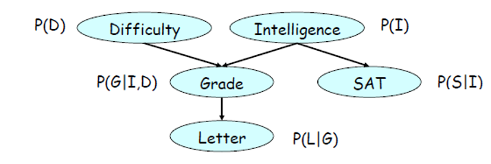
- Difficulty \(D\) is clearly independent of Intelligence \(I\).
- If I already know Intelligence \(I\), knowing the Grade \(G\) wouldn’t add anything to knowing SAT \(S\). It is “independent”.
- But, if I don’t know Intelligence \(I\), knowing the Grade \(G\) would really help knowing something about SAT. So, it is “dependent”.
- So, \(S⊥G|I\), in other words, \(S\) is independent of \(G\) on the condition of knowing \(I\).
Bayesian Networks
- Represent the relationship between variables in terms of conditional independencies
- “Kind of” conveys the idea of how one variable causally influences another, but not always (causality is a complex and disputed notion)
- This is done with a directed acyclic graph (DAG) representation
- Every node has attributed to it a probability distribution conditioned on its parent nodes
- What is most interesting about that is the possibility to decompose the joint probability distribution. For example:
\[ P(D,I,G,S,L) = P(D)P(I)P(G|I,D)P(S|I)P(L|G) \]
- Why is this good? Each distribution can (in principle) be elaborated or trained separately!
- However, we also need to be sure about the conditional independencies
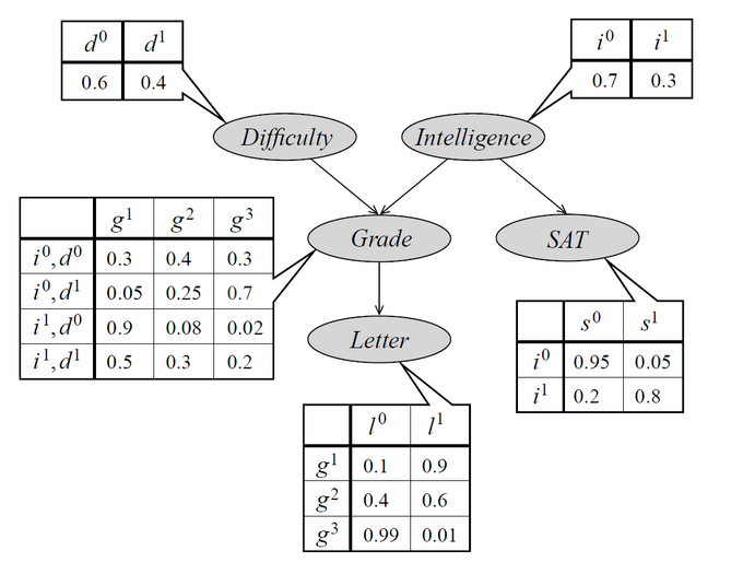
Inferences
- What’s the probability of a recommendation letter given that a student’s SAT is \(s^0\)?
- This means obtaining \(P(L|s^0)\) through the variable elimination algorithm
\[ P(L|s^0) = \frac{P(L,s^0)}{P(s^0)} = \sum_{D,I,G}\frac{P(D,I,G,L,s^0)}{P(s^0)} \] Applying the BN decomposition:
\[ P(L|s^0)= \frac{1}{P(s^0)}\sum_{D,I,G}P(D)P(I)P(G|I,D)P(s^0|I)P(L|G) \]
Calculating \(P(s^0)\):
\[ P(s^0) = \sum_{I}P(s^0,I) = \sum_{I}P(s^0|I)P(I) = P(s^0|i^0)P(i^0) + P(s^0|i^1)P(i^1) = 0.95\times0.7 + 0.2\times0.3 \]
Now, back to \(P(L|s^0)\), let’s eliminate variable \(D\):
\[ P(L|s^0)=\frac{1}{P(s^0)}\sum_{I,G}P(I)P(s^0|I)P(L|G)\sum_{D}P(D)P(G|I,D) \]
This gives us a table \(\tau_1(G,I)=\sum_{D}P(D)P(G|I,D)\)
Now, we eliminate \(I\):
\[ P(L|s^0) = \frac{1}{P(s^0)}\sum_{G}P(L|G)\sum_{I}P(s^0|I)P(I)\tau_1(G,I) \]
which gives us a table \(\tau_2(G)=\sum_{I}P(s^0|I)P(I)\tau_1(G,I)\)
Finally, we eliminate \(G\):
\[ P(L|s^0) = \frac{1}{P(s^0)}\sum_{G}P(L|G)\tau_2(G) \]
We thus get two numbers, \(P(L=l^0|s^0)\) and \(P(L=L=l^1|s^0)\), which would indicate the probability of each outcome.
BNs in Python
- A nice example is implemented with the sorobn library