11.1 Model Types

Objectives

What type of model for what type of data?

• Describe how a Random Forest makes predictions
• Describe how a linear model makes predictions
• Compare and contrast linear and tree models

Setting Up

import pandas as pd
import numpy as np
from sklearn.model_selection import train_test_split
from sklearn.tree import DecisionTreeRegressor, plot_tree, export_text
from sklearn.metrics import mean_absolute_error, accuracy_score, mean_absolute_percentage_error
import plotly.express as px
import plotly.io as pio
pio.templates.default = "plotly_white"

data = pd.read_csv("../../static/data/ames/ames_home_sales.csv")

data['sale_price'] = data.eval("Sale_Price / 1000")
ames = data.query('Gr_Liv_Area < 4000 and Sale_Condition == "Normal"')

ames_train, ames_test = train_test_split(ames, random_state=42, test_size=0.2)
print(f"Training set size: {len(ames_train)} homes")
print(f"Test set size: {len(ames_test)} homes")

Training set size: 1929 homes
Test set size: 483 homes

def evaluate(y_true, y_pred):
    return pd.Series({
        'MAE': mean_absolute_error(y_true, y_pred),
        'MAPE': mean_absolute_percentage_error(y_true, y_pred),
    })

Increasing Depth -> Overfitting

feature_columns = ['Latitude', 'Longitude']
error_data = []
for max_depth in range(2, 30, 2):
    model = DecisionTreeRegressor(max_depth=max_depth, random_state=42).fit(
        X=ames_train[feature_columns],
        y=ames_train['sale_price'])
    
    train_preds = model.predict(ames_train[feature_columns])
    test_preds = model.predict(ames_test[feature_columns])
    error_data.append(dict(
        evaluate(ames_train['sale_price'], train_preds).to_dict(), max_depth=max_depth, dataset='train'))
    error_data.append(dict(
        evaluate(ames_test['sale_price'], test_preds).to_dict(), max_depth=max_depth, dataset='test'))

error_df = pd.DataFrame(error_data)
px.line(error_df, x='max_depth', y='MAE', color='dataset', range_y=[0, 50])

Random Forests Reduce Overfitting

from sklearn.ensemble import RandomForestRegressor
error_data = []
for max_depth in range(2, 30, 2):
    model = RandomForestRegressor(max_depth=max_depth, random_state=42).fit(
        X=ames_train[feature_columns],
        y=ames_train['sale_price'])

    train_preds = model.predict(ames_train[feature_columns])
    test_preds = model.predict(ames_test[feature_columns])
    error_data.append(dict(
        evaluate(ames_train['sale_price'], train_preds).to_dict(), max_depth=max_depth, dataset='train'))
    error_data.append(dict(
        evaluate(ames_test['sale_price'], test_preds).to_dict(), max_depth=max_depth, dataset='test'))

error_df = pd.DataFrame(error_data)
px.line(error_df, x='max_depth', y='MAE', color='dataset', range_y=[0, 50])

A Random Forest has many trees.

model = RandomForestRegressor(max_depth=3, random_state=42, n_estimators=5).fit(
    X=ames_train[feature_columns],
    y=ames_train['sale_price'])
len(model.estimators_)

5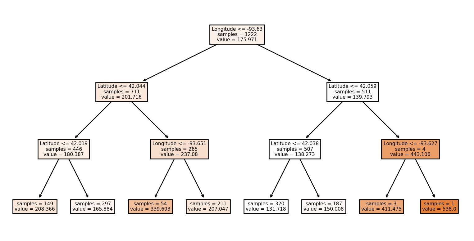

plot_tree(model.estimators_[0], feature_names=feature_columns, filled=True, impurity=False);

Show all 5 trees:

for tree in model.estimators_:
    display(plot_tree(tree, feature_names=feature_columns, filled=True, impurity=False))

[Text(0.5, 0.875, 'Longitude <= -93.63\nsamples = 1222\nvalue = 175.971'),
 Text(0.25, 0.625, 'Latitude <= 42.044\nsamples = 711\nvalue = 201.716'),
 Text(0.125, 0.375, 'Latitude <= 42.019\nsamples = 446\nvalue = 180.387'),
 Text(0.0625, 0.125, 'samples = 149\nvalue = 208.366'),
 Text(0.1875, 0.125, 'samples = 297\nvalue = 165.884'),
 Text(0.375, 0.375, 'Longitude <= -93.651\nsamples = 265\nvalue = 237.08'),
 Text(0.3125, 0.125, 'samples = 54\nvalue = 339.693'),
 Text(0.4375, 0.125, 'samples = 211\nvalue = 207.047'),
 Text(0.75, 0.625, 'Latitude <= 42.059\nsamples = 511\nvalue = 139.793'),
 Text(0.625, 0.375, 'Latitude <= 42.038\nsamples = 507\nvalue = 138.273'),
 Text(0.5625, 0.125, 'samples = 320\nvalue = 131.718'),
 Text(0.6875, 0.125, 'samples = 187\nvalue = 150.008'),
 Text(0.875, 0.375, 'Longitude <= -93.627\nsamples = 4\nvalue = 443.106'),
 Text(0.8125, 0.125, 'samples = 3\nvalue = 411.475'),
 Text(0.9375, 0.125, 'samples = 1\nvalue = 538.0')]

[Text(0.5, 0.875, 'Latitude <= 42.046\nsamples = 1220\nvalue = 175.782'),
 Text(0.25, 0.625, 'Longitude <= -93.679\nsamples = 870\nvalue = 157.211'),
 Text(0.125, 0.375, 'Latitude <= 42.035\nsamples = 166\nvalue = 202.216'),
 Text(0.0625, 0.125, 'samples = 139\nvalue = 208.156'),
 Text(0.1875, 0.125, 'samples = 27\nvalue = 175.668'),
 Text(0.375, 0.375, 'Latitude <= 42.018\nsamples = 704\nvalue = 146.404'),
 Text(0.3125, 0.125, 'samples = 127\nvalue = 177.624'),
 Text(0.4375, 0.125, 'samples = 577\nvalue = 139.294'),
 Text(0.75, 0.625, 'Longitude <= -93.651\nsamples = 350\nvalue = 222.943'),
 Text(0.625, 0.375, 'Longitude <= -93.656\nsamples = 57\nvalue = 356.969'),
 Text(0.5625, 0.125, 'samples = 11\nvalue = 456.043'),
 Text(0.6875, 0.125, 'samples = 46\nvalue = 324.915'),
 Text(0.875, 0.375, 'Longitude <= -93.628\nsamples = 293\nvalue = 196.432'),
 Text(0.8125, 0.125, 'samples = 223\nvalue = 208.485'),
 Text(0.9375, 0.125, 'samples = 70\nvalue = 157.707')]

[Text(0.5, 0.875, 'Longitude <= -93.63\nsamples = 1220\nvalue = 175.311'),
 Text(0.25, 0.625, 'Latitude <= 42.049\nsamples = 719\nvalue = 199.083'),
 Text(0.125, 0.375, 'Latitude <= 42.019\nsamples = 488\nvalue = 180.977'),
 Text(0.0625, 0.125, 'samples = 145\nvalue = 204.302'),
 Text(0.1875, 0.125, 'samples = 343\nvalue = 170.709'),
 Text(0.375, 0.375, 'Longitude <= -93.652\nsamples = 231\nvalue = 239.068'),
 Text(0.3125, 0.125, 'samples = 48\nvalue = 343.917'),
 Text(0.4375, 0.125, 'samples = 183\nvalue = 213.309'),
 Text(0.75, 0.625, 'Latitude <= 42.058\nsamples = 501\nvalue = 139.836'),
 Text(0.625, 0.375, 'Latitude <= 42.038\nsamples = 492\nvalue = 137.218'),
 Text(0.5625, 0.125, 'samples = 306\nvalue = 130.876'),
 Text(0.6875, 0.125, 'samples = 186\nvalue = 147.326'),
 Text(0.875, 0.375, 'Longitude <= -93.626\nsamples = 9\nvalue = 281.956'),
 Text(0.8125, 0.125, 'samples = 6\nvalue = 353.931'),
 Text(0.9375, 0.125, 'samples = 3\nvalue = 152.4')]

[Text(0.5, 0.875, 'Longitude <= -93.63\nsamples = 1201\nvalue = 175.178'),
 Text(0.25, 0.625, 'Latitude <= 42.044\nsamples = 694\nvalue = 198.241'),
 Text(0.125, 0.375, 'Latitude <= 42.019\nsamples = 419\nvalue = 176.474'),
 Text(0.0625, 0.125, 'samples = 143\nvalue = 209.576'),
 Text(0.1875, 0.125, 'samples = 276\nvalue = 160.354'),
 Text(0.375, 0.375, 'Longitude <= -93.652\nsamples = 275\nvalue = 231.549'),
 Text(0.3125, 0.125, 'samples = 54\nvalue = 344.494'),
 Text(0.4375, 0.125, 'samples = 221\nvalue = 206.175'),
 Text(0.75, 0.625, 'Latitude <= 42.057\nsamples = 507\nvalue = 142.491'),
 Text(0.625, 0.375, 'Longitude <= -93.619\nsamples = 499\nvalue = 139.288'),
 Text(0.5625, 0.125, 'samples = 230\nvalue = 132.315'),
 Text(0.6875, 0.125, 'samples = 269\nvalue = 145.077'),
 Text(0.875, 0.375, 'Longitude <= -93.624\nsamples = 8\nvalue = 371.656'),
 Text(0.8125, 0.125, 'samples = 7\nvalue = 397.322'),
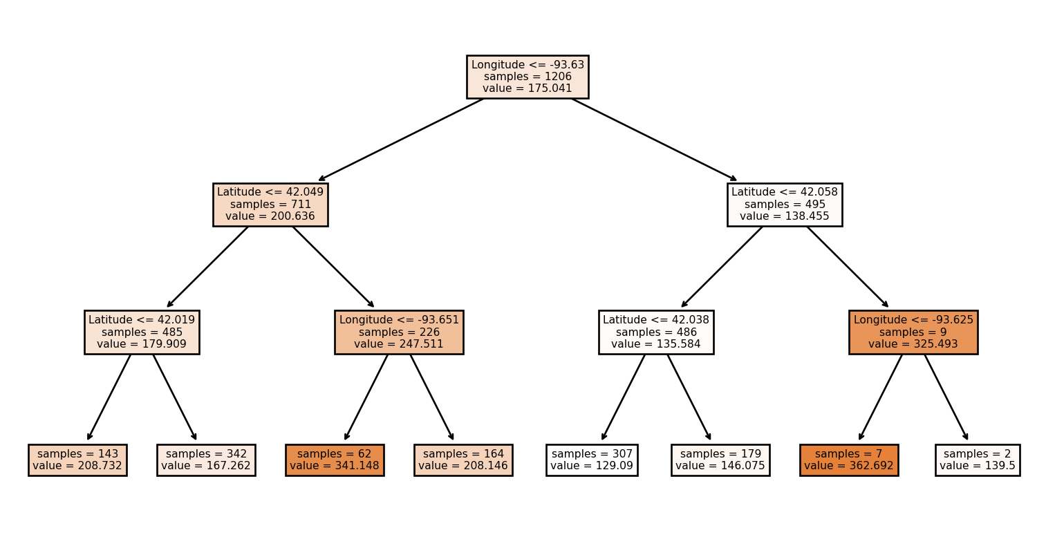
 Text(0.9375, 0.125, 'samples = 1\nvalue = 115.0')]

[Text(0.5, 0.875, 'Longitude <= -93.63\nsamples = 1206\nvalue = 175.041'),
 Text(0.25, 0.625, 'Latitude <= 42.049\nsamples = 711\nvalue = 200.636'),
 Text(0.125, 0.375, 'Latitude <= 42.019\nsamples = 485\nvalue = 179.909'),
 Text(0.0625, 0.125, 'samples = 143\nvalue = 208.732'),
 Text(0.1875, 0.125, 'samples = 342\nvalue = 167.262'),
 Text(0.375, 0.375, 'Longitude <= -93.651\nsamples = 226\nvalue = 247.511'),
 Text(0.3125, 0.125, 'samples = 62\nvalue = 341.148'),
 Text(0.4375, 0.125, 'samples = 164\nvalue = 208.146'),
 Text(0.75, 0.625, 'Latitude <= 42.058\nsamples = 495\nvalue = 138.455'),
 Text(0.625, 0.375, 'Latitude <= 42.038\nsamples = 486\nvalue = 135.584'),
 Text(0.5625, 0.125, 'samples = 307\nvalue = 129.09'),
 Text(0.6875, 0.125, 'samples = 179\nvalue = 146.075'),
 Text(0.875, 0.375, 'Longitude <= -93.625\nsamples = 9\nvalue = 325.493'),
 Text(0.8125, 0.125, 'samples = 7\nvalue = 362.692'),
 Text(0.9375, 0.125, 'samples = 2\nvalue = 139.5')]

Each tree makes different predictions

• It was trained on a different subset of the data
• It was trained on a different subset of the features at each split

predictions = [tree.predict(ames_train[feature_columns].values) for tree in model.estimators_]
predictions = pd.DataFrame(predictions).T
predictions.columns = [f"Tree {i}" for i in range(len(predictions.columns))]
predictions.head()

	Tree 0	Tree 1	Tree 2	Tree 3	Tree 4
0	131.717607	139.294034	130.875931	132.314868	129.090174
1	131.717607	139.294034	130.875931	132.314868	129.090174
2	165.883551	175.668367	170.709185	160.354198	167.262236
3	208.365563	177.624237	204.302481	209.576263	208.732229
4	150.007986	139.294034	147.325621	145.077258	146.075060

To make a prediction

• Each tree makes a prediction
• The predictions are averaged

predictions.mean(axis=1).head()

0    132.658523
1    132.658523
2    167.975507
3    201.720155
4    145.555992
dtype: float64

Value of Diversity

I looked and there before me
was a great multitude that no one could count,
from every nation, tribe, people and language,
standing before the throne.

Revelation 7:9, as quoted in Calvin’s “From Every Nation”

• Random Forests work because they combine diverse perspectives (from different training data, different choices)
• Reflects value of diversity in God’s Kingdom (see also Rev 5:9, 1 Cor 12, etc.)

Linear Models

Fit a Linear Model

from sklearn.linear_model import LinearRegression

feature_columns = ['Gr_Liv_Area'] # we'll add more later
linreg = LinearRegression().fit(
    X=ames_train[feature_columns],
    y=ames_train['sale_price'])
print(f"Intercept: {linreg.intercept_:.2f}")
print(f"Coef: {linreg.coef_[0]:.2f}")

Intercept: 15.98
Coef: 0.11

Prediction equation: \[\text{Sale Price} = 15.98 + 0.11 \times \text{Gr Liv Area}\]

Aside: you may have seen this in stats class

• Stats often asks: “What is the relationship between living area and sale price?”
• Machine learning asks: “How can I predict sale price?”

What computations can a linear model do?

• Trees: only simple conditional logic
  • example: if Gr_Liv_Area <= 2000 then go right else go left
    • (may be <= or >, depending on implementation)
  • predict the average of the training data at the leaf
• Linear models
  • add up terms
  • each term: multiply some feature by a constant (“coefficient”)

Example

First test set house:

test_liv_area = ames_test['Gr_Liv_Area'].iloc[0]
test_liv_area

1008

So we predict:

linreg.intercept_ + linreg.coef_[0] * test_liv_area

124.78893753303895

Actual was:

ames_test['sale_price'].iloc[0]

131.0

Do remodeled homes sell for more?

Year Remod/Add: Remodel date (same as construction date if no remodeling or additions) (from dataset documentation)

ames_train['remodeled'] = ames_train['Year_Remod_Add'] != ames_train['Year_Built']

px.scatter(ames_train, x="Gr_Liv_Area", y="sale_price", color="remodeled", trendline="ols")

Conditional Logic: Simple Conditions

How could a linear model treat remodeled homes differently from non-remodeled?

if remodeled:
  Sale_Price = intercept_remodeled + coef_sqft * Gr_Liv_Area
else:
  Sale_Price = intercept_other + coef_sqft * Gr_Liv_Area

Solution: indicator variables

Sale_Price = 
   intercept_other 
   + coef_sqft      * Gr_Liv_Area
   + coef_remodeled * (1 if remodeled)

Indicator Variables

Sale_Price = 
   intercept_other 
   + coef_sqft      * Gr_Liv_Area
   + coef_remodeled * (1 if remodeled)

feature_columns = ['Gr_Liv_Area', 'remodeled']
linreg = LinearRegression().fit(
    X=ames_train[feature_columns],
    y=ames_train['sale_price'])
print(f"Intercept: {linreg.intercept_:.2f}")
print(f"coef_sqft: {linreg.coef_[0]:.2f}")
print(f"coef_remodeled: {linreg.coef_[1]:.2f}")

Intercept: 21.46
coef_sqft: 0.11
coef_remodeled: -16.11

More than two categories

Bldg Type (Nominal): Type of dwelling
       1Fam Single-family Detached  
       2FmCon   Two-family Conversion; originally built as one-family dwelling
       Duplx    Duplex
       TwnhsE   Townhouse End Unit
       TwnhsI   Townhouse Inside Unit

px.scatter(ames_train, x="Gr_Liv_Area", y="sale_price", color="Bldg_Type", trendline="ols")

One-Hot Encoder

• Input: a column with N categories
• Output: N columns, one per category, with 1 if that category is present, 0 otherwise

from sklearn.preprocessing import OneHotEncoder
one_hot = OneHotEncoder(sparse_output=False)
one_hot.fit(ames_train[['Bldg_Type']])
one_hot.categories_

[array(['Duplex', 'OneFam', 'Twnhs', 'TwnhsE', 'TwoFmCon'], dtype=object)]

pd.DataFrame(
    one_hot.transform(ames_train[['Bldg_Type']]),
    columns=one_hot.categories_).head()

	Duplex	OneFam	Twnhs	TwnhsE	TwoFmCon
0	0.0	1.0	0.0	0.0	0.0
1	0.0	1.0	0.0	0.0	0.0
2	0.0	1.0	0.0	0.0	0.0
3	0.0	1.0	0.0	0.0	0.0
4	0.0	1.0	0.0	0.0	0.0

Preprocessing multiple columns

from sklearn.compose import make_column_transformer
transformer = make_column_transformer(
    ('passthrough', ['Gr_Liv_Area']),
    (OneHotEncoder(sparse_output=False), ['Bldg_Type']),
    remainder='drop')
transformer.set_output(transform='pandas')
transformer.fit_transform(ames_train)

	passthrough__Gr_Liv_Area	onehotencoder__Bldg_Type_Duplex	onehotencoder__Bldg_Type_OneFam	onehotencoder__Bldg_Type_Twnhs	onehotencoder__Bldg_Type_TwnhsE	onehotencoder__Bldg_Type_TwoFmCon
2025	1396	0.0	1.0	0.0	0.0	0.0
2039	1196	0.0	1.0	0.0	0.0	0.0
1143	1677	0.0	1.0	0.0	0.0	0.0
1537	3447	0.0	1.0	0.0	0.0	0.0
2589	884	0.0	1.0	0.0	0.0	0.0
...	...	...	...	...	...	...
1934	1008	0.0	1.0	0.0	0.0	0.0
1263	1253	0.0	1.0	0.0	0.0	0.0
1303	928	0.0	1.0	0.0	0.0	0.0
1490	1127	0.0	1.0	0.0	0.0	0.0
987	1567	0.0	1.0	0.0	0.0	0.0

1929 rows × 6 columns

Putting it all together

from sklearn.pipeline import make_pipeline
model = make_pipeline(
    make_column_transformer(
        ('passthrough', ['Gr_Liv_Area']),
        (OneHotEncoder(sparse_output=False), ['Bldg_Type']),
        remainder='drop'),
    LinearRegression())
model.fit(ames_train, ames_train['sale_price'])

Pipeline(steps=[('columntransformer',
                 ColumnTransformer(transformers=[('passthrough', 'passthrough',
                                                  ['Gr_Liv_Area']),
                                                 ('onehotencoder',
                                                  OneHotEncoder(sparse_output=False),
                                                  ['Bldg_Type'])])),
                ('linearregression', LinearRegression())])

In a Jupyter environment, please rerun this cell to show the HTML representation or trust the notebook.
On GitHub, the HTML representation is unable to render, please try loading this page with nbviewer.org.

What does the model look like?

Prediction equation: \[\text{Sale Price} = -5.61 + 0.11 \times \text{Gr Liv Area} + -34.00 \times \text{Bldg Type 1Fam} + 20.31 \times \text{Bldg Type 2FmCon} + 6.51 \times \text{Bldg Type Duplx} + 42.10 \times \text{Bldg Type TwnhsE}\]

What predictions does it make?

train_predictions = model.predict(ames_train)
evaluate(ames_train['sale_price'], train_predictions)

MAE     31.667456
MAPE     0.192769
dtype: float64

test_predictions = model.predict(ames_test)
evaluate(ames_test['sale_price'], test_predictions)

MAE     32.479024
MAPE     0.195997
dtype: float64